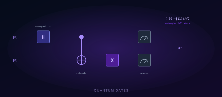
In Part 1 of this series we established that quantum computers use qubits — particles that can exist in superposition, encoding 0 and 1 simultaneously. We saw a variational quantum circuit containing Hadamard gates, rotation gates, and CNOT gates, and noted that these are the trainable operations at the heart of quantum machine learning. But what do those gates actually do? How does a Hadamard gate create superposition, and why does a CNOT gate produce entanglement?
This article opens the hood. By the end you will have a clear mental model of how quantum gates manipulate qubit states — and why that manipulation is computationally extraordinary.
Gates as Rotations in State Space
In classical computing, a logic gate takes one or more bits and produces a fixed output: AND, OR, NOT. Quantum gates differ in two fundamental ways.
First, all quantum gates are reversible. Given the output, you can always reconstruct the input. This is not a design choice — it is a consequence of quantum mechanics itself. The mathematics describing quantum evolution is inherently invertible.
Second, quantum gates are rotations. The state of a single qubit can be visualised as a point on the surface of a unit sphere called the Bloch sphere. The north pole represents |0⟩; the south pole represents |1⟩; points on the equator represent superpositions of both. A quantum gate is a rotation that moves this point around the sphere.
This geometric picture is more than a metaphor. Every single-qubit gate corresponds to a specific rotation around one of the sphere’s axes. Understanding which rotation does what is the foundation of circuit design.
The Hadamard Gate: Creating Superposition
The most important single-qubit gate is the Hadamard gate, written as H. As Part 1 showed, every qubit in a variational circuit typically begins with one.
H rotates the north pole |0⟩ to the equator — creating a state of exactly equal superposition: a 50/50 probability of measuring 0 or 1. Applied twice, H undoes itself and the qubit returns to |0⟩. This self-reversing property is not a coincidence; it reflects the fact that rotating 180° twice returns you to the start.
The practical consequence: H gives quantum algorithms access to all possible inputs at once. Rather than evaluating a function for each input one at a time, a quantum computer with H-initialised qubits probes all inputs simultaneously — a property called quantum parallelism.
The Pauli Gates: Flips and Phase Shifts
The Pauli family — X, Y, Z — are the three fundamental rotations of the Bloch sphere.
The Z gate deserves particular attention. Its output — adding a negative sign to |1⟩ — seems invisible, since measuring the qubit still yields 0 or 1 with the same probabilities. The phase only becomes observable when combined with subsequent gates that create interference. This is exactly how quantum algorithms work: carefully orchestrated phase relationships cancel out wrong answers and reinforce correct ones.
CNOT: The Two-Qubit Gate That Creates Entanglement
The CNOT (Controlled-NOT) gate operates on two qubits — a control and a target. The rule is simple: if the control is |0⟩, leave the target alone; if the control is |1⟩, flip the target.
As a classical truth table, this is unremarkable. The quantum version changes everything. When the control qubit is in superposition — say, the equal superposition produced by H — the CNOT gate does not pick one branch. It processes both simultaneously. The result is a joint state that cannot be written as two independent qubits. The two particles are entangled.
The Bell State: Entanglement from Two Gates
The canonical demonstration of entanglement uses exactly two gates applied to two qubits starting in |00⟩.
The result — (|00⟩ + |11⟩)/√2 — is called a Bell state, and it is maximally entangled. Measure q₁ and find 0: you instantly know q₂ is also 0. Find 1: q₂ is 1. The two qubits never disagree, regardless of the distance between them.
For quantum machine learning, entanglement is not a curiosity — it is a resource. Entangled qubits encode correlations between features of a dataset that would require exponentially many parameters to represent classically. When a variational quantum circuit creates and manipulates entanglement, it is exploring a feature space that no classical network can efficiently replicate.
From Gates to Algorithms
Every quantum algorithm is a carefully designed sequence of these operations. Grover’s algorithm uses H gates to initialise superposition, a phase oracle to mark the target state, and a sequence of reflections using H and Z gates to amplify the probability of finding the correct answer in √N steps instead of N.
In Part 3 of this series, we will trace Grover’s algorithm step by step — following a single search problem through the full circuit and watching the probability of the correct answer grow from 1/N to near 1, in just a handful of gate applications.
Quantum gates are not magic. They are precise rotations in a well-defined mathematical space. The power emerges not from any single gate, but from the structure of what they do together — amplifying signal, cancelling noise, and exploiting correlations that exist nowhere in classical computation.
Sources & Further Reading
- Quantum Computation and Quantum Information (10th Anniversary Edition). Cambridge University Press (2010)
- Elementary Gates for Quantum Computation. Physical Review A 52, 3457; arXiv:quant-ph/9503016 (1995)
- The Physical Implementation of Quantum Computation. Fortschritte der Physik 48; arXiv:quant-ph/0002077 (2000)
Discussion